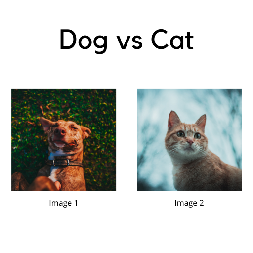
One of the most important applications in Computer Vision is Image Classification. Image Classification is an application of computer vision that serves the purpose of identifying what an image depicts on the basis of its visual content. For example in the following image, it easy for us to identify that image 1 depicts a dog and image 2 depicts a cat. But, the real question is can we provide this ability to a machine?
After a semester of learning Computer Vision and ending up top of my class, I realised one fine day that I knew the theory, but I was not very confident when it came to applying it in practice. So, I headed over to Kaggle and picked up the Plant Pathology 2020 contest. After an initial read through the competition’s details and inspecting the data, I downloaded it and sat down to compete. In the first 15 minutes I realized that the idea of competing seemed a far cry away from my current state, because I did not even have an idea of how I was supposed to pre-process these images. Of course, I could do a few basic operations. But, doing a few basic operations is never enough if you want to build a classifier. After an hour, I was exhausted. I had spent considerable time trying to put to use my theoretical knowledge but was not largely successful in the same. Another issue that I noticed was that I spent too much time surfing the internet for relevant articles that I ended up trying to follow too many different advices and code snippets. Too many cooks did in fact spoil the broth!
A couple of weeks back, I came across this wonderful website called fast.ai and I would highly recommend the reader to head over to that link right now if you want some real, hands-on, straight-to-the-point content. While I have not finished their course yet, I figured the best way to evaluate what I learn would be to practice it! So, this post contains a small, mini-project that I have undertaken as a part of the fast.ai course Practical Deep Learning for Coders (Lecture 1). Apart from writing about my work, I shall also try to explain a few terms that might make it simpler for image classification beginners to follow the content.
Useful links to read before going further ahead
- Should you Kaggle? - A perfect summary of what kaggle is and why you should be a part of it
- The fast.ai website - The home of fast.ai
- Plant Pathology 2020 - FGVC7 Competition Homepage - The competition that provided the dataset used in this mini-project
The Project
In this section, I shall provide a slightly in-depth explanation of the steps I have undertaken while putting my skills to test. Following the steps in this article should help you recreate the project on your own and help you identify key aspects of building an image classifier.
The Zeroth Steps
These include the steps that must be performed prior to writing code to build your classifier.
- Create an account on Kaggle
- Download the Data
- Installing the fast.ai library
If you wish to NOT work on your local system, the use of Kaggle Kernels will be a better choice(one that I would recommend as it helps you make use of the free GPU processing power provided by kaggle). In order to use kaggle kernels, navigate to this link. Click on the New Notebook button on the top right of the page(just below the banner) and follow the remaining steps such as choosing your language, your kernel type(Notebook vs Script) and accelerator(CPU vs GPU vs TPU). At the end, you will have yourself a kaggle notebook.
I have used a kaggle kernel python notebook with a GPU. The fast.ai library is pre-installed in the kaggle kernel. The data from the competition will already have been loaded onto your environment.
Understanding the Problem Statement
The specific objectives of the problem statement(as per the competition) are:
- Classify a given image from testing dataset into an appropriate category
- The categories are healthy, rust, scab and multiple_diseases
- Accurately distinguish between many diseases, sometimes more than one on a single leaf
- Deal with rare classes and novel symptoms
- Address depth perception—angle, light, shade, physiological age of the leaf
Inspecting the Data
Data inspections is an important part of any data science problem. In building an image classifier, it always helps to keep an eye out for preliminary questions like the following about the data:
- What kind of images must be classified?
- What is the size of images? Are they uniform?
- Does the data suffer from imbalance?
From this wonderful kernel by Lex Toumbourou, I was able to identify that:
- All images were not of a uniform size. They were either of 2048x1365 or 1365x20148 dimensions.
- The images were RGB
- The data suffers from imbalance(More on this later)
It is also important to identify the contents of the data. If you are using a kaggle kernel, you would see on the left hand side that the structure is something like this:
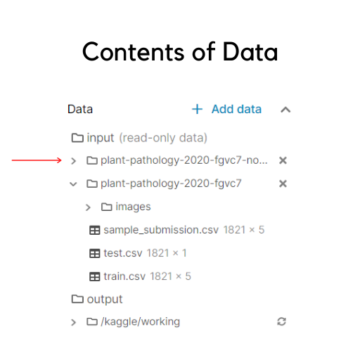
You should ideally have the same structure except the line marked with the red arrow(more on that will be discussed later).
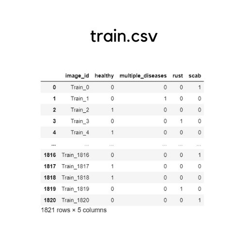
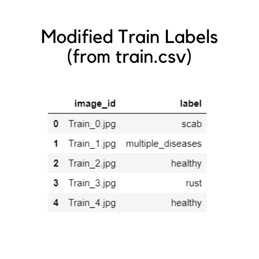
The images folder has all the images. But, it has all train and test images mixed together, without separating them as folders. The sample_submission.csv specifies the format in which you must submit your final predictions for the scorer to evaluate. The test.csv contains only the testing samples that need to be predicted. The train.csv has the labelled samples of training data(depicted beneath).
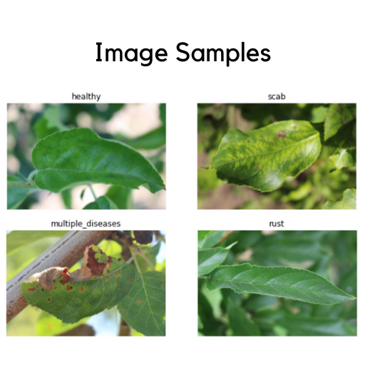
Let’ also have a look on the image samples we have:
If you wish to read a bit about the domain this project deals with, the following links will help:
- The Plant Pathology 2020 challenge dataset to classify foliar disease of apples
- https://en.wikipedia.org/wiki/Apple_scab
- https://www.apsnet.org/edcenter/disandpath/fungalasco/pdlessons/Pages/AppleScab.aspx
- https://extension.psu.edu/apple-diseases-rust
- https://organicgrowersschool.org/ask-ruth-rust-on-apple-tree/
The Issues with the Data
With some preliminary understanding and observation of our data, we find the following relevant issues with it:
- Class Imbalance
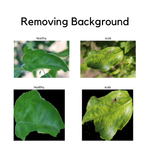
- Background Noise
- Different Lighting Conditions
The problem of class imbalance is very prominent in a lot of datasets. By class imbalance, we simply imply that the number of samples of a particular class in a classification problem is far less in comparison to the number of samples of other classes in the same. For example, in this dataset the class imbalance is depicted as follows:
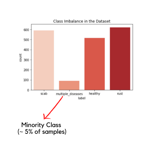
The multiple_diseases class is too small when compared to the other classes and leads to class imbalance.
The problem with class imbalance is that it leads to the accuracy paradox. Suppose you have to classify 100 samples as either being class A or class B. Now, suppose that these 100 samples are distributed as {90: class A, 10:class B}. In such a case, even saying that all 100 samples belong to class A gives you a 90% accuracy. But, is that a good thing to do? What if identifying class B is more important than class A? What if class B is “people with cancer” and class A is “people without cancer”?
Background noise in the context of this problem includes the multiple elements in a given image. For example, an image might have more than one leaf in consideration, have branches etc. The Image Samples pictures above shows plant images that have background noise prevalent in the images. Therefore, it is also necessary to get rid of these backgrounds and select only the leaves from these images. In theory, this might lead to better performance for our models.
Finally, the lighting conditions vary largely in the images. While some are well lit, some are dark. These differences in brightness and contrast are potential causes for a badly performing model.
The Code
The code beneath is a mirror of what I have used in my kaggle notebook. So, if you are trying this project on your local system(or anywhere else), make sure you change the necessary paths.
Loading the libraries
# load the necessary libraries required

import pandas as pd
import matplotlib.pyplot as plt
import seaborn as sns
import numpy as np
import os
import torch
from fastai.vision import *
from fastai.metrics import error_rate
from fastai.basics import *
from fastai.imports import *
from fastai.vision import *
import PIL
from PIL import Image
import re

# beneath are jupyter magic commands
%reload_ext autoreload
%autoreload 2
%matplotlib inline
Setting the Global Variables
# set necessary global variables

BS = 32 # default batch size
PLANTS = '/kaggle/input/plant-pathology-2020-fgvc7' # main folder path
PLANTS_SANS_BKGROUND = '/kaggle/input/plant-pathology-2020-fgvc7-no-background' # background removed images
TRAIN = PLANTS + '/train.csv'
TEST = PLANTS + '/test.csv'
IMAGES = PLANTS + '/images/'
The PLANTS variable contains the path to the original dataset i.e the dataset provided by the competition. The PLANTS_SANS_BKGROUND variable contains the path to a dataset that contains the original images pre-processed in such fashion that the backgrounds are removed. This dataset has been loaded from the publicly released version here created by Victor-Louis De Gusseme.
Process train.csv
The original train.csv file has a separate column for each class(as depicted above). For ease of prediction, I have aggregated all the four columns together and provided one specific label for each image.
# Processing train.csv

def get_label(x):

    label = ''
    if(x.healthy == 1):
        label = label + 'healthy'
    if(x.multiple_diseases == 1):
        label = label + 'multiple_diseases'
    if(x.rust == 1):
        label = label + 'rust'
    if(x.scab == 1):
        label = label + 'scab'

    return label

# load train.csv
train_labels = pd.read_csv(TRAIN)

# Update train_labels dataframe
train_labels['label'] = train_labels.apply(get_label, axis=1)
train_labels = train_labels.drop(['healthy', 'multiple_diseases', 'rust', 'scab'], axis=1)
train_labels['image_id'] = train_labels['image_id']+'.jpg'
train_labels.head()
The output is as follows:
Using fast.ai to build your first classifier
This section is derived from the knowledge I have derived from Practical Deep Learning for Coders and all that I have used here is more or less a mirror-image of what the course teaches, but on a different application. The scope of this post is to only introduce you to the basics of using the fast.ai library. So, if you wish to work more on the same, head over to the course and acquire it directly from the wonderful team behind the fast.ai library.
Moving on, its time to display some more code.
# Data preparation via the fast.ai library
# apply data transformations
tfms = get_transforms(do_flip=True,
flip_vert=True,
p_lighting=0.99,
p_affine=0.75,
max_zoom=2
)
# create the DataBunch object
data = (ImageDataBunch.from_df(path=PLANTS_SANS_BKGROUND,
df=train_labels,
folder=IMAGES,
valid_pct=0.3,
seed=42,
size=224,
ds_tfms=tfms,
bs=BS)
.normalize(imagenet_stats) )
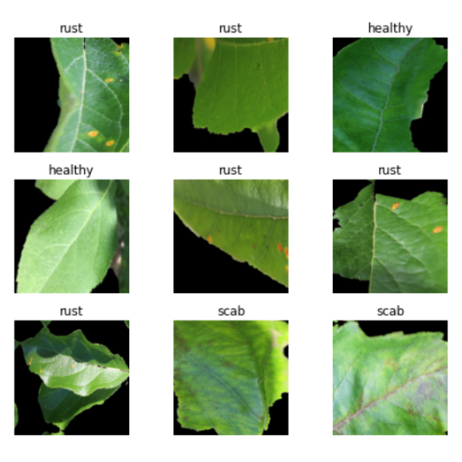
data.show_batch(rows=3, figsize=(7,6))
Meanings of the Terms used above:
- get_transforms()
- Source: https://docs.fast.ai/vision.transform.html
- Purpose: Perform data augmentations(help the model generalize better i.e learn without memorising)
- Arguments used:
- do_flip=True: Flip images randomly with a probability of 0.5
- flip_vert=True: Also applies vertical flips, not just horizontal flips
- p_lighting=0.99: Probability with which a lighting transform is to be applied i.e lighting and contrast change
- p_affine=0.75: Probability with which an affine transform is applied to an image
- max_zoom=2: A random zoom between 1 and 2 will be applied with probability p_affine
- ImageDataBunch.from_df()
- Source: https://docs.fast.ai/vision.data.html#ImageDataBunch
- Purpose: Create the databunch object
- Arguments used:
- path=PLANTS_SANS_BKGROUND: Path to the main dataset
- df=train_labels: The dataframe that has the labels for the training set
- folder=IMAGES: The name of the folder with the images
- valid_pct=0.3: The percentage of data to use for validation
- seed=42: A constant that ensures reproducibility
- size=224: All images are resized to a uniform 224x224 size
- ds_tfms=tfms: Apply the transformations used above
- bs=BS: Batch Size(Decides how many images you want to train at a single time)
- .normalize()
- Normalizes as some channels may be brighter than others.
- Converts to mean of 0 and standard deviation to 1
- data.show_batch() displays a few images from the DataBunch object.
Output:
That’s all for Part 1. Stay tuned for Part 2.